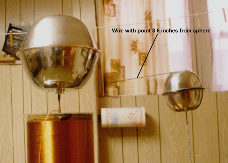
Figure 1. The top terminal of the Tesla coil and a grounded wire.
Abstract:
A new method of analyzing the voltage and current fields generated by Tesla coils allows the author to analyze the electrical fields generated by arcs. This paper presents the data obtained for small arcs to ground.
Introduction:
The development of a new field probe that is able
to measure the voltage and current fields of Tesla coils allows the analysis
of output arcs in a new way. Never before has the ability to see how a
Tesla coil reacts to output arcs been available to this degree of accuracy.
This paper presents the data for small arcs of a few inches. Similar measurements
of much larger arcs have been made but will not be presented here. However,
all of the basic data is similar in larger arcs.
Background:
A small grounded wire was placed a few inches from
the author's Tesla coil to attract output arcs as shown in Figure 1. This
coil was operated at relatively low power for this test to protect nearby
electronic equipment.
Figure 1. The top terminal of the Tesla coil and
a grounded wire.
The potential and current flux fields were received
by an antenna array and the signals were feed to a digital oscilloscope.
Figure 2 shows the antenna array.
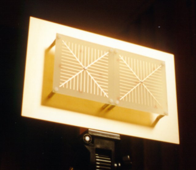
Figure 2. Antenna array.
Figure 3 shows the setup of the test system. The
Tesla coil is on the left and the antenna array is located a safe distance
away on the right.
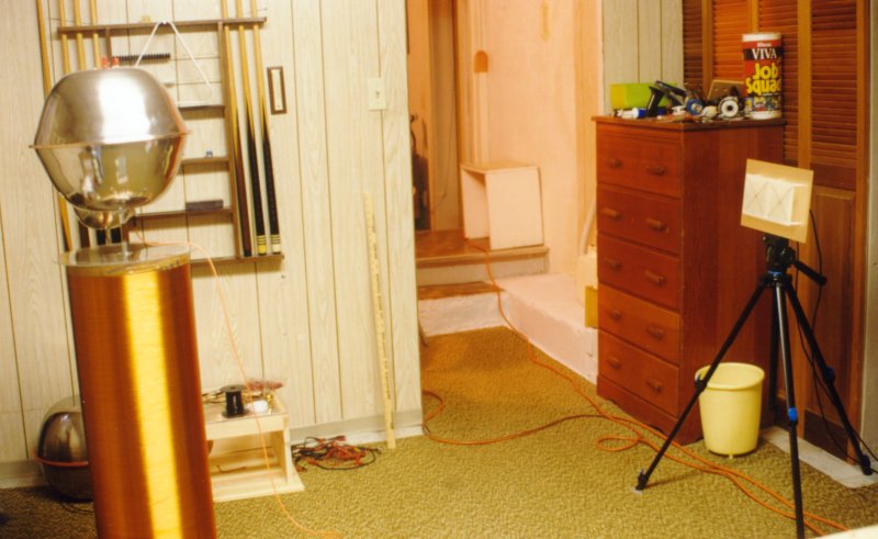
Figure 3. Test setup.
The basic parameters for the Tesla coil are given
below:
Fo = 112000 Hz
Lp = 118.4 uH
Cp = 17.05 nF
K = 0.1475
Ls = 0.0754 H
Cs = 26.78 pF
Spark gap type = Multigap
Results:
Figure 4 shows the voltage and current waveforms
received form the coil during an arc. Note that the arc completely disrupts
the secondary waveforms.
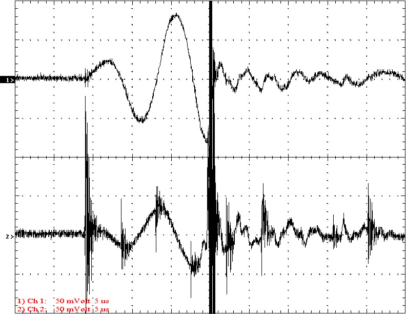
Figure 4. The voltage and current waveforms of an
arc.
Top Trace Voltage 25 kV/div
Bottom Trace Current 1 A/div
Time 5 uS/div
Figure 5 shows the arc event at high speed. The horizontal
time base is only 100 nS/div. Note that the arc is actually oscillating
at about 14 MHz. There are two sharp positive current pulses followed by
a number of oscillations.
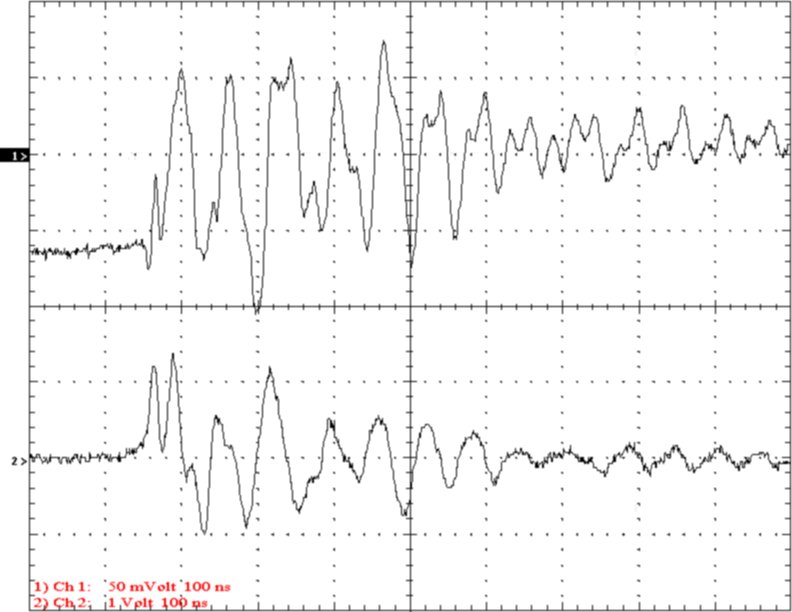
Figure 5. The output arc at high speed.
Top Trace Voltage 25 kV/div
Bottom Trace Current 20 A/div
Time 100 nS/div
To better analyze the arc, the raw data was downloaded into Mathcad and Excel. Figures 6 and 7 show the voltage and current fields of the arc event. It is very interesting to note that the voltage often field exceeds the initial voltage. Other testing has shown that the potential field often approaches twice the original value during arcing. This may contribute to the production of streamers that are longer than the actual terminal voltage would suggest.
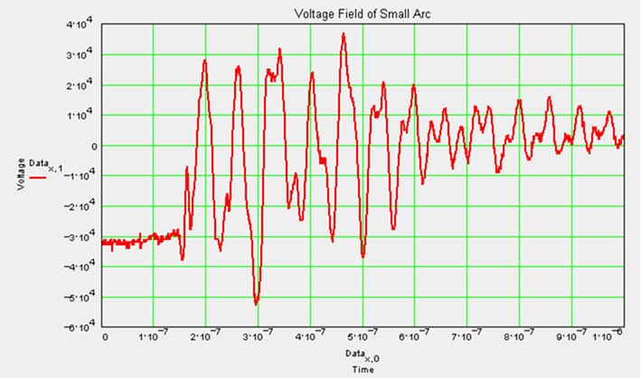
Figure 6. The voltage graph of the arc event. Note
the large negative voltage peak.
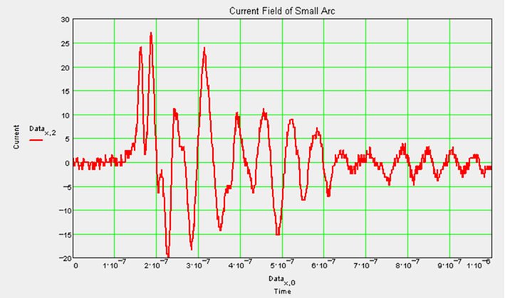
Figure 7. The current graph of the arc event.
Figure 8 shows the instantaneous power of the event.
Note that the energy dissipation is clearly shown in this graph. At 600
nS the oscillations are 90 degrees out of phase and significant power is
no longer being dissipated.
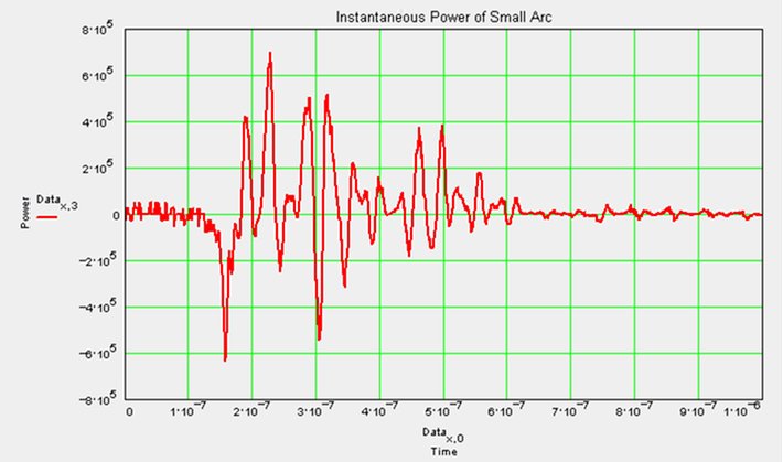
Figure 8. Instantaneous power dissipated in the
event.
Figure 9 shows the sum of the current (integral)
over time. Note that the total charge on the coil changes by ~550 nCoulomb.
The initial voltage was 32000 volts and the secondary capacitance is 26.78
nF giving an initial charge of 857 nCoulomb. Amazingly close considering
the conditions of this measurement. The accuracy improves at higher power.
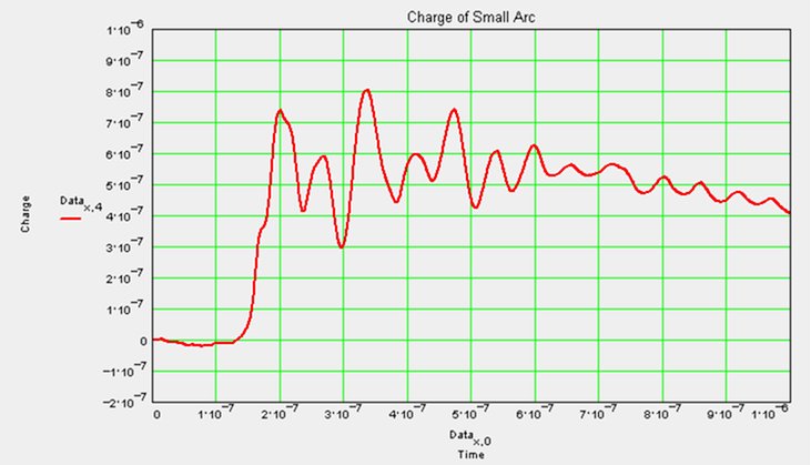
Figure 9. Change in secondary charge (current integrated
over time).
Figure 10 shows the voltage vs. current graph of
the event. Although it is very messy looking, some information can be seen.
The arc is oscillating around a loop suggesting an impedance of ~2000 ohms
for the arc. Other testing shows this to be a rather consistent value for
these arcs to ground.
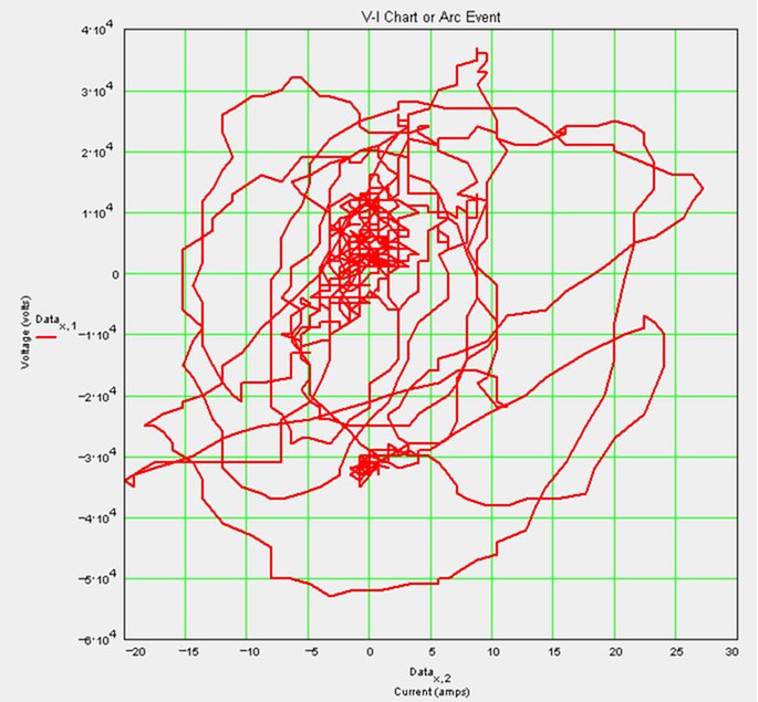
Figure 10. Voltage vs. Current graph.
Figure 11 is The same graph but limited to the first
200 nS of the event. Note that the first two pulses are resistive with
an impedance of ~1 k ohm.
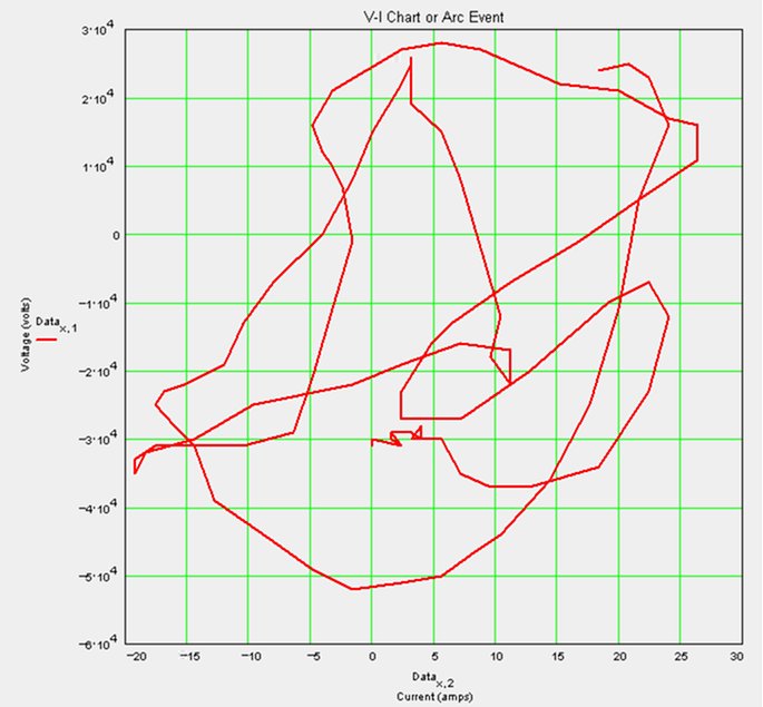
Figure 11. The Voltage vs. Current graph of the
first 500 nS.
Conclusion:
The first data from the new probe system has been presented. There are no real conclusions to be drawn at this time but the theoretical questions raised are many. There are some points that should be mentioned.
1. The arcs to ground seem to present an impedance in the 1 to 3 kohm range consistently.
2. The events last approximately 400 nS. This seems fairly consistent.
3. The first 50 nS of the event seems responsible for doing most of the work in discharging the secondary capacitance.
4. The probe is able to show the change in electric charge in the coil fairly accurately.
5. The characteristics of the arc are very consistent from arc to arc. This indicates that the patterns seen are not random.
6. The output arcs are oscillatory. The frequency seen here is about 14 MHz but variation has been noted in other tests.
7. Often it is seen that the potential field far exceeds the initial voltage during arcing. This may contribute to long streamers that appear to be of higher voltage than the secondary terminal voltage would suggest.