[Published in American Journal of Physics 60, 797-803 (1992)]
Donald G. Bruns
5195 Hearthstone Lane, Colorado Springs, Colorado 80919
(Received 18 October 1991; accepted 19 March 1992)
A low-voltage demonstration Tesla coil using a solid-state photovoltaic relay to replace the conventional spark gap has been analyzed and then built. This relay incorporates an isolated LED to illuminate a silicon photovoltaic stack which drives a bidirectional FET. Component values for the inductances and capacitances have been determined theoretically from measured parameters. Computer simulation by integrating the coupled circuit equations shows excellent agreement with oscilloscope traces. Energy transfer between the primary and secondary circuits is demonstrated, along with continuous secondary oscillations after the primary circuit is interrupted. This low-voltage design is easier to build and diagnose than high-voltage Tesla coils.
Nikola Tesla invented the Tesla coil late in the nineteenth century, exploring many high-power variations in his Colorado Springs laboratory (1). They were all basically air-cored high-frequency transformers, generating very high voltages. Many of his experiments were complicated, using large coils made with heavy copper wires to conduct very high currents. His high-voltage capacitors used hundreds of salt water-filled Leyden jars made from the local Manitou Springs mineral water bottling plant. Tesla documented his achievements with multiple-exposure photographs which show his small wooden building filled with curved sparks up to 40 m in length. Using spark length is how Tesla often diagnosed his experiments.
Tesla's ultimate goal was to generate high enough voltages that he could transmit useful electrical power freely through the atmosphere. One contemporary account claimed he succeeded in sending enough power to energize a bank of light bulbs 40 km away (2). However, he never completed his final and largest experiment on Long Island, New York, which he designed inside a 60-m-high wooden tower. Although lack of funding was the primary reason the tower was torn down, in the light of today's knowledge, it never would have succeeded in the manner he envisioned. While Tesla was advanced for his time, he didn't have electronic diagnostic tools to study his experiments.
Even though Tesla's grandiose plans would not have worked, we remain fascinated with high-voltage Tesla coils. Generating fiery arcs and lighting fluorescent tubes at a distance are always exciting demonstrations. In the last 60 years, instructions for building high-voltage Tesla coils appeared occasionally in popular magazines, journals, newsletters, and books (3-13). A useful instrument in many physics laboratories is the hand-held Tesla coil used to excite gas discharges and find leaks in vacuum systems. There has also been some interest in using very large Tesla coils to test military aircraft with simulated lightning, (14) and using smaller coils to generate electron beams (15). While any of these Tesla coils can be experimental subjects, detailed measurements to compare with theoretical predictions requires sophisticated equipment to deal with high voltages.
A conventional Tesla coil consists of tuned primary and secondary circuits. An interrupter in the primary circuit stimulates oscillations from the charge stored in a large capacitor. The primary circuit interrupter design is critical to maximize power transfer to the secondary circuit. High-power Tesla coils use variations on rotating spark gaps to extinguish the high-voltage spark, (16), a technique that hasn't changed since Tesla used it! This paper replaces that "ancient" element with modern integrated circuit technology. A BOSFET (Bidirectional Output Switch Field Effect Transistor), while not capable of high powers, has the necessary properties which make a demonstration Tesla coil practical. MOSFETs make up the BOSFET, which are combined with an optically coupled LED driver in a small integrated circuit package, manufactured as a photovoltaic relay.(17) It turns on and off quickly, exhibits a low ON-resistance and a high OFF-resistance, and has the capability of transmitting alternating currents. In these respects, it is better than mechanical relays and easier to work with than a spark gap. A Tesla coil with this component can easily be built and diagnosed using a simple oscilloscope. A low-voltage Tesla coil adequately demonstrates all the important theories of a high-power Tesla coil. The example in this paper produces peak secondary voltages of only 20 V, far too small for theatrical demonstrations. The nonlinearities and complications which arise from evaluating a hazardous high-voltage circuit, such as corona leakage, high acoustic and electrical noise levels, and expensive components, are absent from this design. This inexpensive, low-voltage circuit provides easily measurable and reproducible results.
This paper covers classical Tesla coil theory and uses a computer simulation to explain the operation of a small Tesla coil. Excellent agreement between theory and experiment is reached.
The classical Tesla coil theory is presented here. The circuit elements are described, and the differential equations describing the charge are integrated with a short computer program. These results are compared to experimental data in a later section.
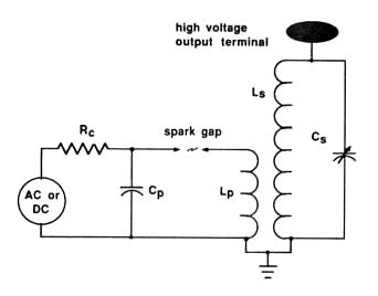
Figure 1 shows the classical Tesla coil configuration. A high-voltage source, often ac, usually with moderately high impedance, charges the primary capacitor Cp up to the spark gap breakdown voltage. The heated air provides a low impedance path as long as a high current flows between the electrodes. In the absence of secondary coupling, the primary current oscillates with a frequency wp determined by the primary circuit components, and decays according to the spark gap resistance. When the capacitor is practically discharged and the primary circuit energy is dissipated, the spark is extinguished and the capacitor recharges. Depending on the spark gap electrode type and separation, this cycle may operate several times during one 60-Hz cycle, or it may only occur once.
Fig. 1. The classical Tesla coil circuit. A high-voltage source charges a capacitor which discharges across a spark gap, stimulating oscillations in the primary and secondary circuits.
When the secondary circuit is included, energy transfers to it at a rate determined by the inductive coupling coefficient k. When all the energy is in the secondary circuit, the process reverses, and the energy begins transferring back to the primary circuit at the same rate. In this case, the optimum design will have the spark gap extinguish just when all the energy is in the secondary circuit. The key design parameters of a Tesla coil optimize this energy transfer.
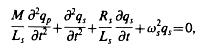
The coupled circuit equations are (18)
![]()
Eq. (1)
and
Eq. (2)
where M = k Ö(LpLs) is the mutual inductance, wp = 1/Ö(LpCp), and ws = 1/Ö(LsCs). With the boundary conditions at t=0 that qs=0, qp= CpV0, dqs/dt=0, and dqp/dt=0, the equations have closed solutions only for Rs and Rp equal to zero. The secondary voltage Vs=qs/Cs consists of two sine waves beating at the difference frequency
![]()
Eq.(3)
with amplitudes depending on Ls, Lp Cs, Cp, and k.(19) When the coupling is such that
![]()
Eq.(4)
for n=0,l,2..., and ws = wp, the two sine waves beat in such a way that the maxima occur simultaneously, and the peak secondary voltage reaches a maximum. This voltage is Vspeak=V0*Ö(Ls/Lp); all the primary circuit energy has transferred to the secondary circuit.
If the tuning ratio wp/ws is not unity and the resistances are not zero, then more complicated equations result, but they can be solved numerically. The larger coupling coefficients, represented by small values of n, result in the highest peak secondary voltages because the transfer of power occurs before much energy is dissipated in the resistances. In these cases, families of curves are required to present all the possibilities of various resistances and tuning ratios; Refs. (18) and (20) give examples.
A short computer program solves the differential equations in the general case of R not equal to 0. While sophisticated Runge-Kutta integration or other routines (21) would work, the solution is smooth enough that simple step-by-step integration with a step size of P/100 is adequate, where P is the oscillation period. The differential equations solutions are expected to be accurate, since the nonlinear losses due to corona leakage and spark gap resistance are absent.
To set up the computer simulation, Eqs. (1) and (2) are integrated once, then the differentials are changed into finite deltas and the integrals into sums. After a little algebra, solving for the circuit current increments leads to
DeltaIp=(Vo-Rp*Ip-SumQp/Cp-M*DeltaIs/DeltaT) *DeltaT/Lp Eq.(5)
and
DeltaIs = ( - Rs*Is - SumQs/Cs - M*DeltaIp/DeltaT)*DeltaT/Ls. Eq.(6)
The computer program first defines the component values, the initial primary voltage, and the integration step size. The coupling coefficient k was used to calculate M. Perfect tuning was assumed, so the values of wp^2 and ws^2 were equal.
Inside a loop incremented by DeltaT, the computer calculated the values of DeltaIp and DeltaIs, then the values were updated by calculating
Ip = Ip + DeltaIp,
SumQp = SumQp + Ip*DeltaT,
Is = Is + DeltaIs,
SumQs=SumQs + Is*DeltaT, and
Time =Time+DeltaT. Eq.(7)
To simulate the BOSFET turn-off, Rp was changed to 1000 W when the time shown in the oscilloscope photos was reached.
The time-dependent values of Vp = SumQp/Cp - V0 and Vs = SumQs/Cs were plotted in real time. Output changes resulting from small changes in any of the parameters were studied, but the results in this paper are from the measured values.
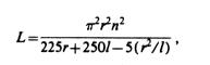
The inductance values and the coupling coefficient in this experiment were calculated from as-built coil dimensions. The capacitances were determined from frequency measurements. The minimum resistances were determined from theoretical considerations, but the effective resistances were used as free parameters in the computer simulation. Table I shows the physical specifications.
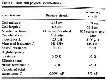
The primary and secondary inductances have a length/diameter ratio large enough so they can be calculated by the Nagaoka formula (22) for closely spaced air solenoids;
Eq. (8)
where n is the number of turns, r the radius in cm, l is the length in cm, and L is given in microhenries. The inductance error is less than 1% at low frequencies. The primary coil dc resistance was too low to measure accurately with a simple multimeter, so it was calculated using a wire resistance table. The secondary coil’s calculated and measured values agreed. The relative impedance change at the operating frequency, however, differs significantly for the two coils. Using the formulas and charts from Ref. 23, the skin depth for copper wire at 148 kHz is approximately 175 microns. The high-frequency impedance of #18 copper is larger by approximately 50%, while for #30 wire, the value is practically unchanged. The proximity effects of a close-wound coil causes a bigger correction, adding about 14% to the secondary coil impedance and about 75% to the primary coil. The final results lead to a primary coil impedance about 2.3 times, and the secondary coil impedance about 1.15 times, the dc value. The minimum primary coil impedance calculates to 0.23 W and the secondary impedance to 33 W.
The actual effective resistance was even larger, determined by fitting the computer simulation to oscilloscope measurements. The primary coil measurement is shown in Fig. 2. The primary and secondary circuits were pulsed individually to determine their resonant frequencies. The BOSFET impedance drives up the effective resistance more than expected; their dc resistance was directly measured at 12 W, but the simulation required 12 for the primary coil. The secondary value agreed better, requiring 45 W to match the measurements. The resistances used in the simulations do affect the decay constants, but do not change the overall curve shapes. The resonant frequency determined by the oscilloscope measurements led to accurate capacitance values. The primary circuit is not tunable, so its resonant frequency is defined as wp. With the primary oscillating and the secondary coil placed about 30 cm away, its variable capacitor could be tuned through its resonant peak. At this distance, mutual coupling between the circuits is small enough not to cause any frequency shifts, but strong enough to provide a measurable secondary circuit signal.
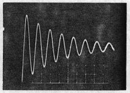
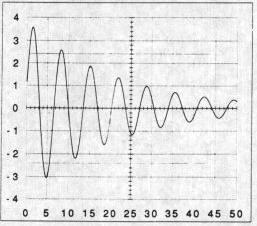
Fig. 2. Primary coil effective resistance measurement. (a) The oscilloscope photograph, (b) a computer simulation. The vertical axis numbers are volts. The bottom axis numbers are microseconds.
The primary capacitance Cp is a single capacitor with a nominal 0.0l-mF component marking. A more precise value was determined by measuring the free oscillation frequency and letting
![]()
Eq. (9)
since both Lp and wp could be determined with only a few percent error. This led to a determination of 0.0091 mF for Cp, only 10% lower than nominal.
In a conventional Tesla coil, the secondary capacitance Cs is the sum of the top electrode capacitance Cs' in parallel with the self-capacitance Cs’’. The self-capacitance is estimated from the chart in Ref. 24; for single layer solenoids, the self-capacitance depends weakly on the length. For most typical Tesla coil geometries, the self-capacitance (in picofarads) equals the diameter in cm. Spherical top electrodes contribute a capacitance equal to Ct = 4per, where r is the top electrode radius. For this demonstration Tesla coil, all of these numbers are too small to produce a low enough frequency for BOSFET operation, so a large tunable capacitor was added in parallel. The secondary circuit capacitance Cs was set by simply tuning that circuit to the primary's resonant frequency.
The coupling coefficient k is calculated for typical Tesla coil geometries using the formula (Ref. 25) for concentric coils,
![]()
Eq. (10)
where
Eq. (11)
np and ns are the number of turns per centimeter on the coil, and
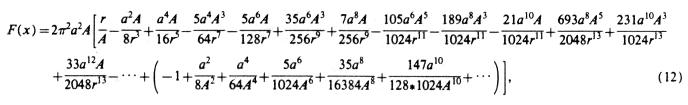
Eq. (12)
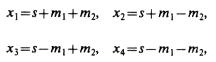
where r^2 = x^2+A^2, s is the center to center distance, a is the radius of secondary coil, A is the radius of primary coil (A> a), 2m1 is the length of secondary coil, 2m2 is the length of primary coil, and all measurements are in centimeters. Knowing Ls and Lp determines k.
While this formula appears complicated, it is the only formula I found which converges for typical Tesla coil geometries and k values. Gray's formula (Ref. 26), while simpler, does not converge for close coupling. The coefficient k is plotted in Fig. 3 over the range used in this experiment. The coupling near s = 10 cm slopes about 0.05 per cm, so a significant error occurs for inaccurate measurements. Nevertheless, the computer simulation shows excellent agreement with the predicted value of k for each experiment.
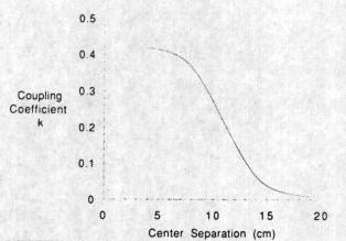
Fig. 3. Calculated coupling coefficient k, using the Tesla coil parameters from Table I and the equations from Ref. 25.
Preliminary experiments were conducted to assist in the design and evaluation of this Tesla coil demonstrator and to provide measurements for comparison with the computer simulation. The BOSFET’s drive circuit was explored for the fastest switching times.
The Tesla coil operating frequency was designed around this switching time.
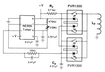
Fig. 4. Tesla coil primary driver schematic. Two dual BOSFET units are used in parallel to replace the spark gap with a low-resistance interrupter.
A switching circuit based on the PVR 1300 solid-state relay with internal BOSFET replaced the spark gap in this demonstration. An isolated LED inside the PVR 1300 illuminates a silicon photovoltaic stack surrounded by a reflective cavity to increase efficiency. The voltage generated by the stack drives internal circuits connected to the BOSFET gate. Since this circuitry is not tied to an external reference voltage, the device can be made to pass alternating currents. When turned on, the BOSFET acts as a nearly pure resistance with practically no offset voltage. When turned off, the device offers over l00-MW resistance. The turn on and off are essentially limited only by the LED drive circuits, so 100 kHz operation is possible. No other solid-state device has this combination of properties over such a wide frequency range.
The Tesla coil master timing was designed around the simple integrated circuit pulser shown in Fig. 4. While the BOSFETs are OFF, the primary capacitor charges through the 2700W resistor Rc. After the 0.0l-mF capacitor Cp is charged, the NE555 pulser triggers the BOSFETs and the primary coil current starts flowing. For the first few microseconds, the BOSFETs have a high and varying resistance, so the circuit simulation starts after this initial period. The Tesla coil was designed with a low enough frequency that this initial time is short compared to one oscillation period. After that, the BOSFET was treated as a constant resistance.
Since the lowest possible ON resistance was important, two dual BOSFET packages were paralleled. The nominal ON-switching time is 18 ms with the maximum recommended 25-mA LED drive current, but this shrinks to about 3 ms with the drive circuit shown in Fig. 4. The actual switching times depend on the BOSFET terminal current; these values are typical at the maximum 400 mA pass currents. The 0.47 mF speed-up capacitor across the 100 W current limiting resistor boosts the initial current into the LEDs. Although high currents are not recommended for long durations, LED damage normally occurs due to thermal problems, and pulses shorter than a few microseconds are safe. The turn-off time was only a few microseconds, which is unimportant in this application. Once the BOSFETs turn on, a low dc ON-resistance of about 1.2 W (for the four units in parallel) is maintained. The OFF-resistance value is not important, but the specifications indicate many megohms are typical.
Experiments were performed to measure the Tesla coil parameters and to provide comparison data for the computer simulation. Excellent agreement is seen.
The case of small coupling, where the coils are just beginning to overlap, corresponds to k values less than about 0.2. Figure 5 shows the oscilloscope traces and the matching computer simulations for two primary beats. Except near the zero crossing voltage, the simulations very closely matched the measured voltages.
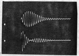
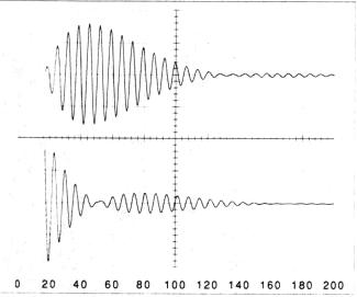
Fig. 5. Tesla coil operation for weak coupling, k=0.072. (a) The oscilloscope photograph, (b) a computer simulation. This value of k corresponds to n=13. Upper trace: Secondary circuit. 5 V/div. Lower trace: Primary circuit, 2 V/div. input 8.7 V; 25-mA LED drive current. The bottom axis numbers are microseconds.
According to Eq. (3), the beat period should be 94 ms for the k=0.072 case. This value agrees well with the Fig. 5 data, even though this calculation is for R = 0. This shows that resistive damping does not significantly affect the oscillation frequencies.
Figure 6 shows the case for centered (s=0) coils, which gives the maximum k value of 0.43. In this case, many beats occur and the simulation is very sensitive to minute changes in the coil parameters. The general form of the traces match surprisingly well, but due to the many zero crossings, the curves do not match in detail. Here, the beat period calculates as 14 ms, but a periodicity of about 16 ms is seen. For large coupling, the resistance values are more important in the equations.
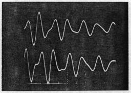
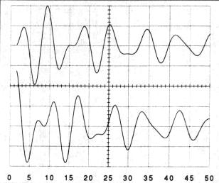
Fig. 6. Tesla coil operation for strong coupling, k=0.43. (a) The oscilloscope photograph, (b) a computer simulation. This value of k corresponds to n = 2. Upper trace: Secondary circuit, 10 V/div. Lower trace: Primary circuit, 2 V/div, input 9.3 V; 29 mA LED drive current. The bottom axis numbers are microseconds.
The most efficient Tesla coil operation occurs when the primary circuit stops oscillating near its beating envelope minima while the total circuit losses are still small. Figure 7 illustrates this; the BOSFETs were turned off just as the primary voltage envelope reached a minimum on its second envelope cycle. Some stray pickup causes the small voltage oscillations in the photograph. The secondary amplitude no longer beats with the primary, but decays normally.
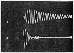
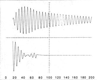
Fig. 7. Tesla coil operation for weak coupling, k=0.072. (a) The oscilloscope photograph, (b) a computer simulation. This value of k corresponds to n = 13. Upper trace: Secondary circuit, 5 V/div. Lower trace: Primary circuit, 2 V/div, input 8.7 V; 25-mA LED drive current. The bottom axis numbers are microseconds. BOSFET turn off occurred at 72 ms.
This demonstration Tesla coil provides a tool to explore various Tesla coil design parameters without dangerous experiments or high-voltage nonlinearities. Excellent theoretical agreement results using measured parameters in a computer simulation. The circuit could use other high-speed switches, but none currently are as convenient and as practical as the BOSFET. Another possibility for a demonstrator uses frequencies so low that ordinary mechanical relays could be used. If the relay's response time is reproducible to 1 ms, then a resonant frequency of 100 Hz could be practical. This very low frequency could be obtained by using a 100-cm radius primary coil with 100 turns and 100 each of 1 mF nonpolarized capacitors in parallel for Cp. The secondary would be similarly scaled to large dimensions. While that approach would be interesting, this solid-state BOSFET design demonstrates the important parameters in a personal, inexpensive unit. The same BOSFET switch could temporarily replace the spark gap in a high-power Tesla coil, permitting tuning and some debugging at lower powers. As long as people are fascinated with high-voltage demonstrations, Tesla coils will be popular, and this demonstration can help them safely learn about them.
The author would like to thank his father, Arnold G. Bruns, for stimulating a life-long interest in Tesla coils by building the author's childhood home on top of the same small hill in Colorado Springs where Tesla's lab was located some 60 years earlier.
Return to Don Bruns home page
Return to Stellar Products home page