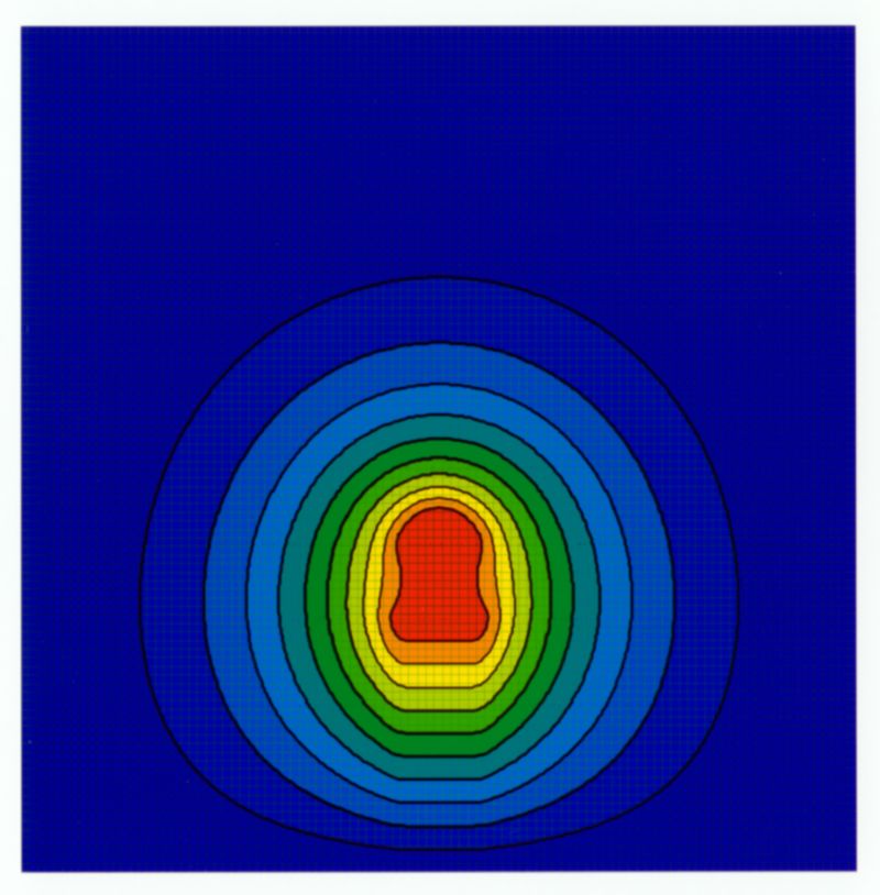
Figure 1. A model of the potential field around the author's Tesla coil.
Abstract:
A new method of analyzing the voltage and current fields generated by Tesla coils is described. This method allows for the accurate measurement of the potential and current of the output through the use of field sensing antennas. This method allows analysis of a coil's output with the following advantages:
1. This method can accurately measure and analyze the characteristics of output arcs, output potential and secondary current in real time.
2. The measurement bandwidth is approximately 100 MHz with phase relationships preserved.
3. The antennas used are inexpensive, easily made, and have no critical or difficult adjustments.
4. There is no contact (electrical or physical) to the coil to disturb the system being measured.
5. The characteristics and design of this system have been analyzed using standard design methods. The principles of operation are well understood.
Hopefully, this new measurement method will allow
revolutionary advances in Tesla coil analysis and design.
Warning and Disclaimer: The author assumes no responsibility for the operation, design, construction, accuracy or safety of the devices described herein. This paper deals with highly experimental amateur equipment used in an extreme electrical environment. Only persons with advanced knowledge of these systems should attempt to experiment with the described devices. Any attempt to reproduce or operate the described devices is at the readers own risk!
Introduction:
In order to understand Tesla coils, the ability to measure basic fundamental current and voltage levels is extremely important. Theories and guesses about Tesla coil operation can never be confirmed or disproved without the ability to make these measurements. The lack of this information is responsible for the widely varying opinions and theories that have surrounded Tesla coil operation from the beginning.
The secondary voltages and currents in Tesla coils are very difficult to measure. The extreme voltages and the sensitivity of the system to external influences render most typical methods useless. Typical high voltage measuring equipment either draws too much current from the secondary or disturbs the tuning of the system. Many methods have been tried and theories abound. However, no truly effective method has been presented to date. Fiber-optic systems can measure top terminal currents and all primary currents and voltages but they cannot directly measure secondary voltage due to the lack of a ground reference. Also, at extreme frequencies, fiber-optic transducers saturate and loose their ability to function properly. Only recently have secondary measurements of current been attempted by fiber optics or by persons within very large top terminals. The results from such basic fundamental measurements have completely changed many very long held beliefs about Tesla coil operation. The only common method to get any idea of the secondary voltage behavior has been with the use of simple wire antennas connected to an oscilloscope. However, the accuracy, frequency response and effectiveness of these systems only allow very rudimentary tests to be performed.
Accurate models now exist that can very accurately predict most Tesla coil parameters. However, the study of output sparks is the last of the fundamental measurements still to be made. This is also the most theoretically difficult measurement to make with any accuracy. The extreme voltages, frequencies, currents, etc. are far beyond any typical measurement method.
This paper describes a system that specifically
addresses all these problems. The author has found a method that appears
to be able to accurately measure the voltage and current fields produced
by Tesla coils. This method presents no unusual loads to the coil, is capable
of up to 100MHz operation, is not limited to any maximum voltage level,
and has very good accuracy.
Background:
During an attempt, by the author, to increase the frequency response of a simple wire antenna connected to an oscilloscope, it was found that the fundamental sensitivity of the antenna could be changed from voltage to current. By properly loading the system, the antenna can loose it's sensitivity to the electrostatic potential field and become sensitive to the current flux field. This phenomenon is not typically known do to its limited usefulness. However, in the case of Tesla coil secondary measurements, this phenomenon can be exploited in a very useful way. If fact, the very high power nature of Tesla coils allows such a method of measurement to work successfully. The author has developed a method, based on this phenomenon that is capable of measuring the electrostatic potential field and the current flux field. These measurements are directly proportional to the actual fields present and can be calibrated to good accuracy.
Since this method uses distant antennas, there are no physical connections to the coil. This eliminates all loading problems. By carefully designing the system, the bandwidth has been extended into the 100MHz region with a very flat frequency response. The sensitivity of the system can be adjusted simply by varying the distance of the antenna from the coil. This allows for coils of any size to be measured. The antennas are always located far enough from the coil to eliminate the concern for equipment damage due to arcing. This system has no critical adjustments, is easy and inexpensive to construct, and is simple to use.
Theory of Operation:
This voltage and current probe's operation is based on the fundamentals of electrostatics. Tesla coils deliver electric charge into a capacitance formed by the top terminal and the self-capacitance of the coil. The primary system and the secondary inductor force electrons into (or out of) the secondary capacitance of the coil. As this capacitance charges, two fields of interest are created.
There is a potential distribution field
that is basically a series of concentric spheres of a given voltage. The
potential near the top terminal is very high while far from the coil the
potential is less. Figure 1 shows a model of this potential field.
Figure 1. A model of the potential field
around the author's Tesla coil.
As the secondary capacitance charges, energy
is stored by raising the potential of the area around the top of the coil.
It is important to realize that no ground is needed for charge to be stored
in the space around the coil. The following equations from electrostatic
theory govern this situation:
Q = C x V = I t
J = V x Q = 1/2 x C x V^2
Where:
Q = Electric charge in Coulombs
C = Capacitance in Farads
V = Electric Potential in Volts
I = Current in Amps
t = Time in seconds
J = Energy in Joules
The second field is the current flux field. As the
area around the sphere is charged, current is forced outward and away from
the top of the coil into the surrounding space. This current density field
is responsible for charging the space around the coil to a given potential.
The following equation from electrostatic theory governs this situation:
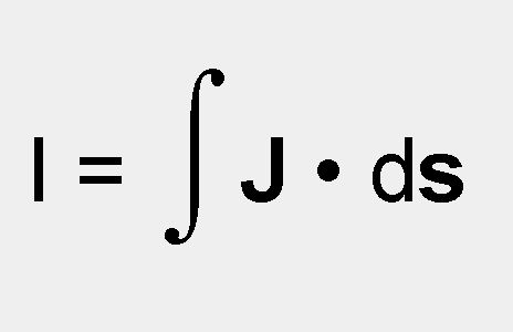
Where:
I = Current in amps
J = Current flux density
s = A section of the enclosed surface
In other words, the total current equals the current flux density integrated over the enclosed surface area (people who care, know what this means).
We now have two fields. The electrostatic potential
field that is proportional to the secondary voltage and the flux density
field that is proportional to the current projected into the space around
the coil.
For those less familiar with electrostatic theory the following should be understood. When electrons are stored in the top terminal the voltage on the terminal increases proportionally (V = Q / C). The current that enters the base of the secondary coil in effect continues to flow into the space around the coil and is reabsorbed back into the surroundings and eventually finds it's way back to the base of the secondary inductor. In other words the current path forms a large circle. From the base of the coil to the top, out word into space, from space to the surroundings and from surroundings back the base of the secondary.
There is a technical detail, the electrons get stored at the top of the coil. However, the electrons in the space around the coil are proportionally forced away into the surroundings so the overall effect is basically as described.
Our goal is to measure the potential or voltage on
the secondary caused by the stored electrons in the top of the coil and
to measure the current flow that is required to get it there.
Design:
In order to detect the fields around the Tesla coil, plane wave antenna arrays are used. There are two antennas, a current-sensing antenna and a voltage-sensing antenna.
The current antenna is a true proportional plane wave current sensor. In order to measure the current flow around the coil, a plane of wires connected to a resistive load of low value senses a section of the area around the coil. The current ratio is simply the ratio of area of the sensor to the area formed by a sphere around the coil. The radius of the sphere is the same as the distance from the coil to the antenna. Since there are other objects and such that bend this field a bit, some fine tuning is needed. For an antenna area of 12.25 square inches and a divider ratio of 1000:1 the distance works out to 62.44 inches (1000 x 12.25 = pi x R^2). The actual distance in the author's case measures out to 65 inches.
The voltage antenna is identical to the current antenna with the exception that instead of a low value resistive load, it has a capacitor as a load. The capacitance between the coil and the antenna and the capacitive load form a voltage divider. The voltage is directly proportional to the coil's secondary voltage. The only unknown is the capacitance value from the secondary to the antenna. Although the near objects affect this capacitance to a fair degree it can still be estimated. However, it is easiest to simply calculate the voltage and adjust the system to achieve calibration. This will be discussed later. Figures 2, 3, and 4 show the antenna arrays.
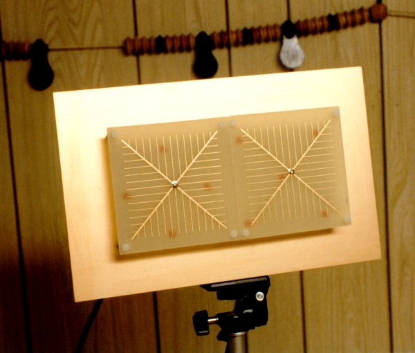
Figure 2. Front of dual antenna array.

Figure 3. Side view. Note that more components have
been added since this photo (R1, R2, And C3).
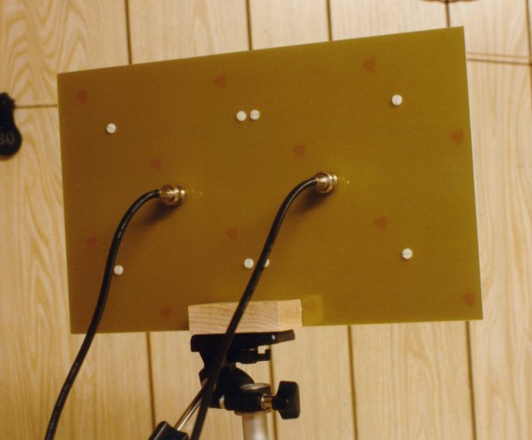
Figures 4. The back showing the BNC connections.

Figure 5. The artwork of the antenna array. The
actual antennas are split into two boards. The area of the wire arrays
is 12.25 square inches or 3.5 inches on a side.
The array is mounted 1 inch away from a 12 x 7.5 inch ground plane made from a sheet of copper clad PC board. The BNC connectors are mounted to the back plane. The components (R1, R2, and C3) are mounted between the back plane and the antennas.
In order to get the signals from the antennas to the oscilloscope input, a coaxial cable is used. This cable represents a transmission line and the antenna system must be designed to take the cable impedance into account. It is also necessary to design the system so that the bandwidth is high and the frequency response is flat. This is extremely important to insure that the signals the oscilloscope receives are correct. This may sound difficult but is actually very easy due to two reasons. The first is that the circuit uses simple components that are not critical. The second is that the author has already designed it :-) Figure 6 shows a Spice model of the voltage and current antennas. Figures 7 and 8 show the outputs and frequency response of the probes.
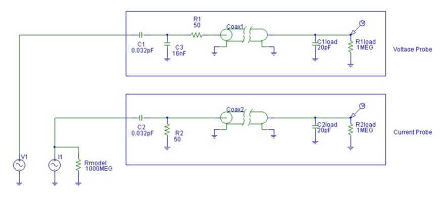
Figure 6. Spice model of the voltage and current
antenna systems.
V1 and I1 represent the Tesla coil output.
Rmodel is required for the spice model to run and
can be ignored.
C1 and C2 represent the capacitance from the Tesla
coil to the antennas.
C3 is the voltage probe load.
R1 is required to compensate for the coax cable.
(Must be 50 ohms to match the cable.)
R2 is the current probe load. (Must be 50 ohms to
match the cable.)
C1, C2, R1load, and R2load represent the oscilloscope's
input impedance. (Tektronix TDS210.)
Basically, the Tesla coil's output represented by Vi and I1 couples to the antennas through a capacitance represented by C1 and C2. C3 and R2 provide voltage and current sensing loads that are transmitted through the 50-ohm impedance coaxial cables to the oscilloscope's input impedance. The frequency response is limited by the oscilloscope's input impedance. If smaller input impedances are available, the frequency response can be extended further. Note that R1 and R2 are critically matched to the impedance of the coaxial cables. The calibration of the current is adjusted by moving the antenna closer to or further from the coil. The calibration of the voltage is adjusted by varying the value of C3. Once the current is known, the secondary voltage can be calculated by the following equation:
Vs = Is x Ls x 2 x pi x Fo
Where:
Vs = The coil's secondary voltage
Is = The coil's secondary current
pi = 3.14159...
Fo = The coil's resonant frequency
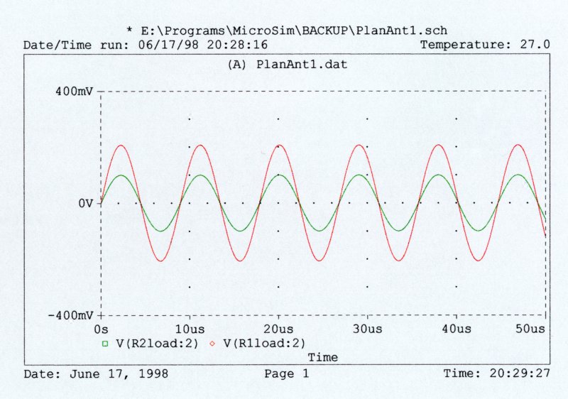
Figure 7. Time domain response.
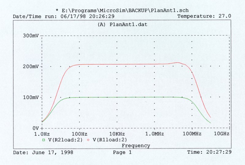
Figure 8. Frequency response.
Construction:
The probe system is very easy to construct. The parts used in the author's system are listed bellow. Parts with special requirements are noted. Most parts can be varied and substituted to some degree. Indeed the system presented may not be optimal or have still other improvements yet to be found. The parts are as follows:
Quan.
Description
2 12 foot,
50 ohm, BNC to BNC coaxial cables to connect the antennas to the oscilloscope.
If extremely long cables are used the system may be affected but in general
any length of 50-ohm cable can be used.
2
51-ohm, surface mount, 1/8 watt resistors. These resistors need to be small
surface mount types to handle the high bandwidth.
1 10nF and some 1nF 50-volt, surface mount capacitors. These need to be high quality surface mount types to insure good performance at very high frequencies. The 1nF capacitors are used to adjust the voltage level.
1 12 x 7.5 inch copper printed circuit board. This serves as a ground plane for the antenna and as the base for everything else.
2 3.5 x 3.5 inch plane antennas as shown. The size and wire layout is not critical but if a different size is used the output voltages will change. The area of each array is 12.25 square inches.
2 BNC panel mount connectors.
8 1-inch plastic spacers and 16 nylon screws. Or anything non-conductive to mount the antennas 1 inch away from the ground plan.
Testing:
Figure 9 shows the author's test setup. The antenna arrays are mounted on a tripod and connected to an oscilloscope shown in Figure 10.
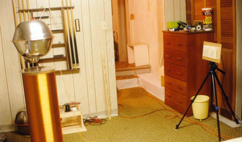
Figure 9. Test setup.
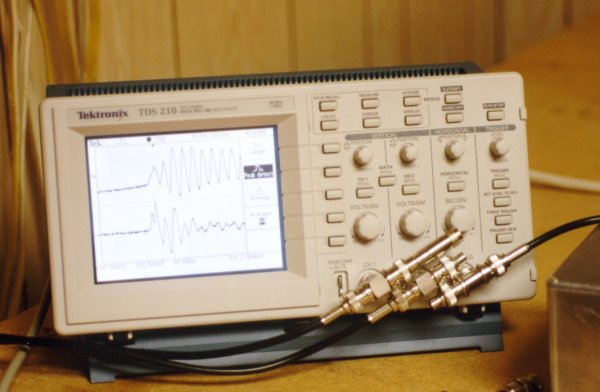
Figure 10. Oscilloscope. (Attenuators shown are
no longer used).
The following figures show various tests done with this system to verify its operation.

Figure 11. A current calibration test.
Channel 1 Current 1A/div Secondary ground fiber-optic
probe
Channel 2 Current 1A/div Plane-wave antenna
Note: this photo is from a prototype system.
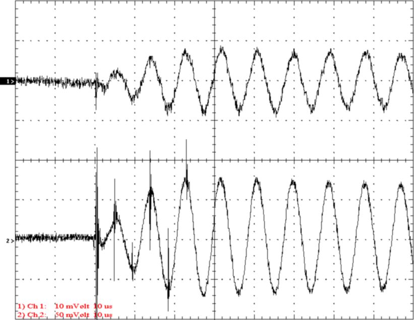
Figure 12. A current calibration test.
Channel 1 Current 1A/div Current into top terminal
fiber-optic probe
Channel 2 Current 1A/div Plane-wave antenna
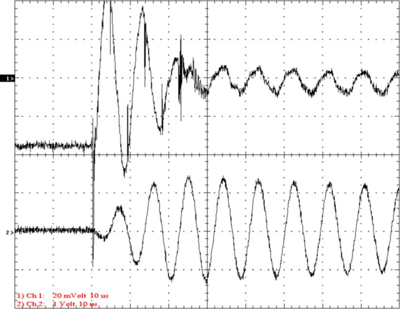
Figure 13. Calibration test.
Channel 1 Voltage 2kV/div Primary capacitor voltage
fiber-optic probe
Channel 2 Voltage 50kV/div Output plane-wave antenna
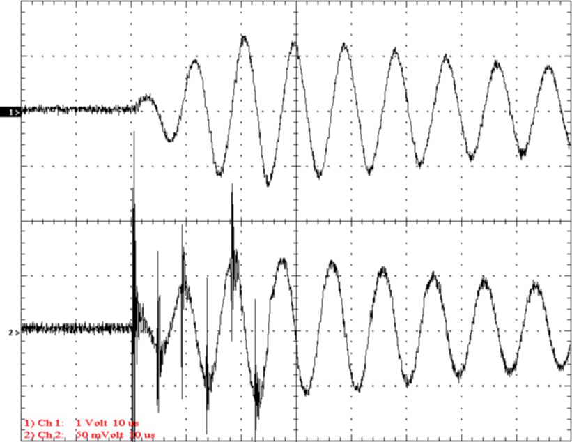
Figure 13. Calibration test. No breakout.
Channel 1 Voltage 50kV/div Plane-wave antenna
Channel 2 Current 1AV/div Plane-wave antenna
The distance of the current antenna was adjusted
until the base current was equal to the current on the current probe antenna.
The capacitance of the Voltage antenna was adjusted so that the voltage
output was equal to the current times the inductance of the secondary multiplied
by the frequency in radians/sec.
Conclusion:
A method for the accurate measurement of the output voltages and currents of Tesla coils has been presented. This system provides major improvements over any previously know methods. This system does not affect the coil, has very high bandwidth, and flat frequency response. This method is theoretically sound and can be used on any similar type of Tesla system regardless of size. This system is not complex and can be easily reproduced. Hopefully, this new measurement method will allow revolutionary advances in Tesla coil analysis and design.